Graph is a connection of nodes with edges. Node is sometimes called as vertex, and edges is sometimes called branch.
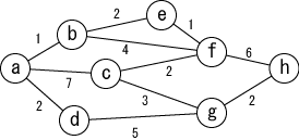
An example graph is shown in Figure 1. In the figure, nodes are represened by letters and circles, and edges are represented by lines coneecting nodes. The number near the edge is the weight of the edge.
 |
| Figure 1: Example of Graph |
The graph of Figure 1 can be represented by the adjacency matrix in Table 1. Here, each element of the matrix is its weight if there is an edge between the nodes, or "-" if there is none. We also assume that the weight between the same nodes is 0.
| Table1: Adjacency Matrix | |||||||||||||||||||||||||||||||||||||||||||||||||||||||||||||||||||||||||||||||||
|
A number of cities and the road distances connecting them are given. Write a program that finds the shortest route from the starting city to the destination city.
$N$ $R$
$A_1$ $B_1$ $L_1$
$A_2$ $B_2$ $L_2$
$\quad\cdots$
$A_R$ $B_R$ $L_R$
$S$ $D$
The first line contains 2 integers $N$ and $R$ which represent the number of cities, and the number of roads connecting those cities, respectively.
$1 \leqq N \leqq 100$
Each of the $R$ lines after the second line contains 3 integers, $A_i$, $B_i$, and $L_i$
$~~$ ($1 \leqq i \leqq R$).
$A_i$ and $B_i$ represent both ends of the $i$-th road, and
$L_i$ represents the distance of the road.
$0 \leqq A_i \leqq N-1$
$0 \leqq B_i \leqq N-1$
The last line contains 2 integers, $S$, $D$ which represent the starting city and the destination city, respectively.
$0 \leqq S \leqq N-1$
$0 \leqq D \leqq N-1$
If the shortest path is found, print it as follows.
On the first line, print an integer representing the distance of the shortest path. And on the next line, print the cities along the shortest path from the starting city to the destination city, with a space between them.
If there are multiple shortest path, one of them should be the answere.
If there is no shortest path, print "no route".
Dijkstra's is an algorithm that finds the shortest path to each node one bye one from the vicinity of the starting node, and gradually expands the range. Can be used when all edge weights are non-negative ($\geqq 0$).
 |
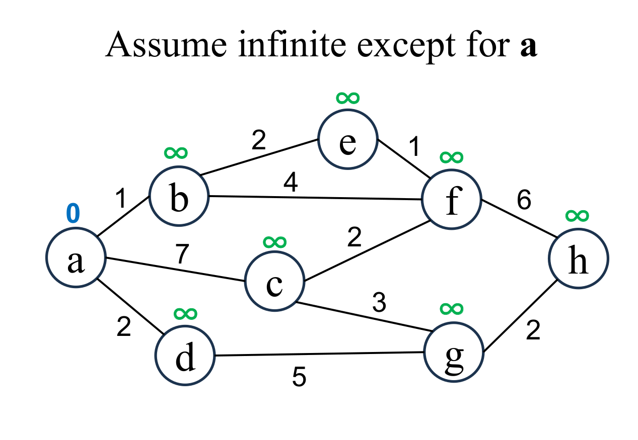
Let's find the shortest path from node a to node h. |
 |
Assume that the shortest distance of each node is "unfixed"
and its value is infinity ($\infty$). Then, assume the shortest distance of the starting node (a) is 0. |
 |
Select the shortest node
(a marked with ☆)
among the "unfixed" nodes. The shortest distance of the selected node (a marked with ☆) is "fixed" to the current value (0). The "fixed" node is separated from "unfixed" nodes by a red boundary line (frontier). |
 |
Calculate the distance of each node (b, c, d ), if and only if the node is "directly connected" from the most recently fixed node (a with ☆), and its "shortest distance" is "unfixed". If the result is less than current value, update it (b → 1, c → 7, d → 2). Edges that update the shortest distance of unfixed nodes across the boundary are expressed by light blue arrows. |
 |
Select the shortest node
(b marked with ☆)
among the "unfixed" nodes. The shortest distance of the selected node (b marked with ☆) is "fixed" to the current value (1). If there are multiple nodes with the shortest distance value, it doesn't matter which one you choose. |
 |
Calculate the distance of each node (e, f), if and only if the node is "directly connected" from the most recently fixed node (b with ☆), and its "shortest distance" is "unfixed". If the result is less than current value, update it (e → 3, f → 5). |
 |
Select the shortest node
(d marked with ☆)
among the "unfixed" nodes. The shortest distance of the selected node (d marked with ☆) is "fixed" to the current value (2). |
 |
Calculate the distance of node (g), if and only if the node is "directly connected" from the most recently fixed node (d with ☆), and its "shortest distance" is "unfixed". If the result is less than current value, update it (g → 7). |
 |
Select the shortest node
(e marked with ☆)
among the "unfixed" nodes. The shortest distance of the selected node (e marked with ☆) is "fixed" to the current value (3). |
 |
Calculate the distance of node (f), if and only if the node is "directly connected" from the most recently fixed node (e with ☆), and its "shortest distance" is "unfixed". If the result is less than current value, update it (f → 4). |
 |
Select the shortest node
(f marked with ☆)
among the "unfixed" nodes. The shortest distance of the selected node (f marked with ☆) is "fixed" to the current value (4). |
 |
Calculate the distance of each node (c, h), if and only if the node is "directly connected" from the most recently fixed node (f with ☆), and its "shortest distance" is "unfixed". If the result is less than current value, update it (c → 6, h → 10). |
 |
Select the shortest node
(c marked with ☆)
among the "unfixed" nodes. The shortest distance of the selected node (c marked with ☆) is "fixed" to the current value (6). |
 |
Calculate the distance of each node (g), if and only if the node is "directly connected" from the most recently fixed node (g with ☆), and its "shortest distance" is "unfixed". The shortest distance of g is not updated, becase the computed result(9 is not less than the current value (7). |
 |
Select the shortest node
(g marked with ☆)
among the "unfixed" nodes. The shortest distance of the selected node (g marked with ☆) is "fixed" to the current value (7). |
 |
Calculate the distance of each node (h), if and only if the node is "directly connected" from the most recently fixed node (g with ☆), and its "shortest distance" is "unfixed". If the result is less than current value, update it (h → 9). |
 |
Select the shortest node
(h marked with ☆)
among the "unfixed" nodes. The shortest distance of the selected node (h marked with ☆) is "fixed" to the current value (9). |
 |
The shortest distance (9) from a to h and shortest path (a → d → g → h) are found. |
Consider the example below to explain why Dijkstra's algorithm works correctly.

The above figure is immediately after "node b is fixed and the estimated distance of nodes e and f are updated".
There are 3 types of node status.
Dijkstra's algorithm asserts that "the shortest node (d) among the unfixed nodes can be fixed with the current value (2)". And it is clear from the fact that "all edge weights are non-negative" in the graph Dijkstra's targets.
Consider the "unfixed" nodes on the right side of the boundary line. The "unfixed but estimated" nodes (c, d, e, f) hold the shortest distance via the current "fixed" nodes (a, b). Then, the shortest node (d) among the "unfixed but estimated" nodes (c, d, e, f) has the shortest distance even including "unfixed and infinity ($\infty$)" nodes (g, h). Because all edge weights are non-negative, going to d through the current "unfixed" nodes is far.

In other words, the shortest distance from a to d is currently estimated correctly and can be fixed at the current value.

Thinking like this, we can see that Dijkstra's algorithm claims something very obvious.
It is important to focus on the boundary line (frontier) between the "fixed" nodes and "unfixed" nodes. The "unfixed but estimated" nodes are connected directly with some "fixed" nodes. The shortest "unfixed but estimated" node (d) cannot be shorter via other unfixed nodes. Therefore, its true minimum value has already been found.
The shortest distance of one node is fixed in one loop. Since this is repeated for $n$ nodes, the complexity of this iterative operation is $O(n)$.
Once the shortest distance to a node is fixed, update the distance estimates for each node connected to that node. The maximum number nodes connected to a node is $n-1$, so the complexity of this operation is $O(n)$.
So the total complexity is $O(n) \times O(n) = O(n^2)$.
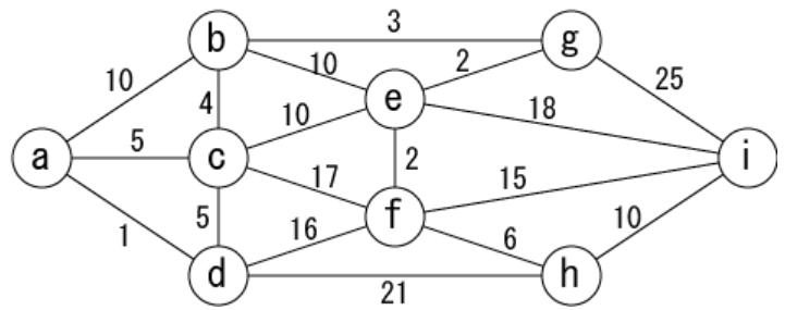
In the following graph, answer the distance of the shortest route from node a to node i.
a: Start node
Run dijkstraPath.py on the following data and measure the computation time.
| dijkstra.py |
#!/usr/bin/env python
import queue

G = [{}]

def setNode(n):
  global G
  G = [{} for i in range(n)]
def addEdge(s,t,w):
  global G
  G[s][t]=w
def solve(s,t):
  global G
  fixed = {}
  q = queue.PriorityQueue()
  q.put((0,s))
  while q.empty() == False:
    w,x = q.get()
    if x in fixed: continue;
    fixed[x] = w
    if x == t: return w
    for y in G[x]:
      if (y in fixed) == False:
        q.put((w + G[x][y], y))
  return None


n,m = map(int,input().split())
setNode(n)
for i in range(m):
  s,t,w = map(int,input().split())
  addEdge(s,t,w)
  addEdge(t,s,w)
src, dst = map(int,input().split())
print(solve(src,dst))
|
| Execution Log of dijkstra.py |
$ ./dijkstra.py < route03.data |
When updating the distance to a node, record the previous node in via[]. Once the shortest distance to the destination node is fixed, the shortest path can be found by tracing the transit nodes in reverse order.
| dijkstraPath.py |
#!/usr/bin/env python
import queue

G = [{}]

def setNode(n):
  global G
  G = [{} for i in range(n)]
def addEdge(s,t,w):
  global G
  G[s][t]=w
def getRoute(via,s,t):
    r = [t]
    y = t
    while y != s:
        y = via[y]
        r.append(y)
    r.reverse()
    return r
def solve(s,t):
  global G
  fixed = {}
  via = {}
  q = queue.PriorityQueue()
  q.put((0,s,None))
  while q.empty() == False:
    w,x,prev = q.get()
    if x in fixed: continue;
    fixed[x] = w
    via[x] = prev
    if x == t:
        return w, getRoute(via,s,t)
    for y in G[x]:
      if (y in fixed) == False:
        q.put((w + G[x][y],y,x))
  return None, None


n,m = map(int,input().split())
setNode(n)
for i in range(m):
  s,t,w = map(int,input().split())
  addEdge(s,t,w)
  addEdge(t,s,w)
src, dst = map(int,input().split())
d,r = solve(src,dst)
print(d)
print(r)
|
| Execution log of dijkstraPath.py |
$ ./dijkstraPath.py < route03.data |
The slow Java program that simply implements Dijkstra's algorithm is as follows.
| Dijkstra.java |
import java.util.*;
public class Dijkstra {
    public static void main(String[] args) {
        Scanner sc = new Scanner(System.in); // read from Standard Input
        int n = sc.nextInt(); // number of nodes
        int m = sc.nextInt(); // number of edges
        int[][] mat = new int[n][n]; // Adjacency matrix of node connections
        for (int i=0; i<n; i++) // initialize the matrix
            for (int j=0; j<n; j++)
                mat[i][j] = (i==j) ? 0 : -1;
        for (int i=0; i<m; i++) { // read edges
            int s = sc.nextInt(); // one node of the edge
            int t = sc.nextInt(); // another node of the edge
            int w = sc.nextInt(); // weights
            mat[s][t] = mat[t][s] = w;
        }
        int src = sc.nextInt(); // start node
        int dst = sc.nextInt(); // destination node
        int d = dijkstra(mat,src,dst);
        System.out.println((d==Integer.MAX_VALUE) ? "no route" : d);
    }
    public static int dijkstra(int[][] mat,int src,int dst) {
        int n = mat.length;
        int[] distance = new int[n]; // shortest distance to nodes
        boolean[] fixed = new boolean[n]; // shortes distance is fixed?
        for (int i=0; i<n; i++) { // initialize nodes
            distance[i] = Integer.MAX_VALUE; // initial distance is infinity
            fixed[i] = false;   // shortest distance is unfixed
        }
        distance[src] = 0;      // distance of start node is 0
        while (true) {
            int x = minIndex(distance,fixed); // shortest node in unfixed nodes
            if (x == dst) return distance[x]; // find the answer
            if (x < 0 || distance[x]==Integer.MAX_VALUE) return Integer.MAX_VALUE; // unconnected graph
            fixed[x] = true; // node x is fixed.
            for (int y=0; y<n; y++) { // for each node
                if (mat[x][y]>0 && !fixed[y]) { // if y is directly connected with x and y is unfixed
                    int d2 = distance[x]+mat[x][y];// calculate distance of y via x
                    // if shorter, update the shortest distance of y
                    if (d2 < distance[y]) distance[y] = d2;
                }
            }
        }
    }
    // returns index of minimum distance[] whose fixed[] is false
    static int minIndex(int[] distance,boolean[] fixed) {
        int idx = -1;
        for (int i=0; i<fixed.length; i++) {
            if (!fixed[i]) // unfixed
                if (idx < 0 || distance[idx] > distance[i]) idx = i; // index of shortest node
        }
        return idx;
    }
}
|
| Execution log of Dijkstra.java |
$ javac Dijkstra.java |
In "Dijkstra.java", node connections are kept in memory as a 2-dimensional array, so large data may cause an Out-of-Memory Exception and terminate program execution. In that case, expand the heap memory of the java virtual machine with the -Xms option of java command.
| route13.data(part) |
62500 124906 0 1 15 0 250 58 1 2 79 1 251 1 2 3 144 ...(omitted)... |
| Expand heap memory when Dijkstra.java runs |
$ javac Dijkstra.java |
Let's change the program that is also shows the shortest path.
Record the previous node in via[] when updating the shortest distance for each node.
| Change DijkstraPath.java Output of " diff -c Dijkstra.java DijkstraPath.java" |
*** Dijkstra.java	Wed Jul 12 11:44:25 2023
--- DijkstraPath.java	Wed Jul 12 11:55:19 2023
***************
*** 1,3 ****
  import java.util.*;
! public class Dijkstra {
      public static void main(String[] args) {
--- 1,4 ----
  import java.util.*;
! public class DijkstraPath {
!     static int[] via; // previous node updating distance
      public static void main(String[] args) {
***************
*** 19,21 ****
          int d = dijkstra(mat,src,dst);
!         System.out.println((d==Integer.MAX_VALUE) ? "no route" : d);
      }
--- 20,40 ----
          int d = dijkstra(mat,src,dst);
!         if (d == Integer.MAX_VALUE) {
!             System.out.println("no route");
!         } else {
!             System.out.println(d);
!             StringBuilder sb = new StringBuilder();
!             for (int x: getRoute(src, dst)) sb.append(x + " ");
!             System.out.println(sb.toString());
!         }
!     }
!     static ArrayList<Integer> getRoute(int src, int dst) {
!         ArrayList<Integer> r = new ArrayList<>();
!         r.add(dst);
!         int x = dst;
!         while (x != src) {
!             x = via[x];
!             r.add(x);
!         }
!         Collections.reverse(r);
!         return r;
      }
***************
*** 25,26 ****
--- 44,46 ----
          boolean[] fixed = new boolean[n]; // shortes distance is fixed?
+ 	via = new int[n]; // previous node
          for (int i=0; i<n; i++) { // initialize nodes
***************
*** 28,29 ****
--- 48,50 ----
              fixed[i] = false;   // shortest distance is unfixed
+ 	    via[i] = -1; // previous node is unknown
          }
***************
*** 39,41 ****
                      // if shorter, update the shortest distance of y
!                     if (d2 < distance[y]) distance[y] = d2;
                  }
--- 60,62 ----
                      // if shorter, update the shortest distance of y
!                     if (d2 < distance[y]) { distance[y] = d2; via[y] = x; }
                  }
|
| Execution log of DijkstraPath.java |
$ javac DijkstraPath.java |
For a sparse graph with many nodes, such as route13.data, try expanding the head memory when running "DijkstraPath.java". In some environment, it can be calculated, albeit slowly.
| Execution time of DijkstraPath.java for route13.data CPU:Ryzen 5900HX, Memory: DDR4 32GB |
$ time (java -Xms16g DijkstraPath < route13.data >/dev/null) |
In Dijkstra's algorithm, when dealing with sparse graphs (that is, graphs with fewer edges than the number of nodes), it is expected that the calculation speed will be increased by the following measures. Although the complexity order does not change.
The computational complexity of Priority First Seach is:
$\quad$ "for each of $n$ nodes"
$\quad$$\quad$ "to retrieve the shortest node from the heap"
$\quad$$\quad$ and
$\quad$$\quad$ "to update the distance of nodes directly connected by the most recently fixed node",
where
"for each of $n$ nodes" : $O(n)$
"to retrieve the shortest node from the heap": $O(\log n)$
"to update the distance of nodes directly connected by most recently fixed node": $O(n)$ ← can be regarded as a constant for sparse graphs.
The practical execution time is expected to be
$O(n) \times O( \log n + \mbox{Constant}) = O(n \log n)$ .
Priority Queue is a data structure called a "heap" that allows access to specific data in $O(\log n)$.
The Java program of Priority First Search written using the PriorityQueue class is as follows.
| PFSPath.java |
import java.util.*;
public class PFSPath {
    static ArrayList<Node> graph = new ArrayList<>();
    public static void main(String[] args) {
	Scanner sc = new Scanner(System.in); // read from Standard Input
	int n = sc.nextInt(); // nubmer of nodes
	int m = sc.nextInt(); // nubmer of edges
	for (int i=0; i<n; i++)
	    graph.add(new Node(i, Integer.MAX_VALUE)); // instanciate each node
	for (int i=0; i<m; i++) { // read edges
	    int s = sc.nextInt(); // one node of the edge
	    int t = sc.nextInt(); // another node of the edge
	    int w = sc.nextInt(); // weights
	    graph.get(s).addEdge(t,w); // add edge from s to t
	    graph.get(t).addEdge(s,w); // add edge from t to s
	}
	Node src = graph.get(sc.nextInt());	// start node
	Node dst = graph.get(sc.nextInt());	// destination node
	int d = dijkstra(src, dst);
	if (d ==Integer.MAX_VALUE) {
	    System.out.println("no route");
	} else {
	    System.out.println(d);
	    StringBuilder sb = new StringBuilder();
	    for (Node x: getRoute(src, dst)) sb.append(x.id + " ");
	    System.out.println(sb.toString());
	}
    }
    public static int dijkstra(Node src, Node dst) {
	HashSet<Node> fixed = new HashSet<>(); // fixed node
	src.d = 0;	// distance of start node is 0
	var queue = new PriorityQueue<Node>();
	queue.add(src);
	while (queue.size() > 0) {
	    Node x = queue.poll(); // get minimum node from queue
	    assert !fixed.contains(x);
	    if (x == dst) return x.d; // find the answer
	    fixed.add(x); // set node x as fixed
	    for (Map.Entry<Integer,Integer> entry: x.edges.entrySet()) { // each edge from node x
		Node y = graph.get(entry.getKey()); // edge's endpoint
		int w = entry.getValue(); // edge's weights
		int d2 = x.d + w; // distance to y via x
		if (fixed.contains(y) || d2 >= y.d) continue; // do nothing if fixed or further
		if (queue.contains(y)) queue.remove(y); // remove y from queue
		y.d = d2; // update distance to y
		y.via = x; // set the previous node of y is x
		queue.add(y);  // add y into queue
	    }
	}
	return Integer.MAX_VALUE; // unconnected
    }
    static ArrayList<Node> getRoute(Node src, Node dst) { // shortest path from src to dst
	ArrayList<Node> r = new ArrayList<>();
	r.add(dst); // start from dst
	Node x = dst;
	while (x != src) { // trace back to src
	    x = x.via;
	    r.add(x);
	}
	Collections.reverse(r); // reverse the list (src->dst)
	return r;
    }
    static class Node implements Comparable<Node> { // node
	int id;    // node identity
	int d;     // distance
	Node via;  // previous node
	HashMap<Integer, Integer> edges; // edge: (edge's endpoint, weights)
	public Node(int id, int d) {
	    this.id = id;
	    this.d = d;
	    edges = new HashMap<>();
	}
	void addEdge(int t, int w) { edges.put(t, w); }
	public int compareTo(Node x) { return d - x.d; }
    }
}
|
| Execution log of PFSPath.java |
$ java PFSPath < route03.data |
Let's run "PFSPath.java" against data representing a sparse graph with many nodes, say "route13.data" Unlike the case of "DijkstraPath.java", the answer can be obtained with "small memory consumption" and "fast".
| Execution time of PFSPath.java for route13.data CPU:Ryzen 5900HX, Memory: DDR4 32GB |
$ time (java PFSPath < route13.data >/dev/null) |
Dijkstra's algorithm cannot solve when there are edges with negative weights in the graph. In such cases, use the Bellman-Ford algorithm to solve.